Betweenness （介数） ¶

介数¶

本示例演示如何使用自定义的调色板来可视化顶点和边的介数。我们分别使用 betweenness() 和 edge_betweenness() 方法，并演示它们在标准 Krackhardt Kite 图以及 Watts-Strogatz 随机图上的效果。

首先我们导入 igraph 和一些用于绘图等的库

import random
import matplotlib.pyplot as plt
from matplotlib.cm import ScalarMappable
from matplotlib.colors import LinearSegmentedColormap, Normalize
import igraph as ig

接下来，我们定义一个函数，用于在 Matplotlib 轴上绘制图。我们根据介数值设置每个顶点和边的颜色和大小，并在侧面生成一些颜色条，以查看它们如何相互转换。我们使用 Matplotlib 的 Normalize 类来确保我们的颜色条范围是正确的，并使用 igraph 的 rescale() 来将介数重新缩放到 [0, 1] 区间

def plot_betweenness(g, ax, cax1, cax2):
    '''Plot vertex/edge betweenness, with colorbars

    Args:
        g: the graph to plot.
        ax: the Axes for the graph
        cax1: the Axes for the vertex betweenness colorbar
        cax2: the Axes for the edge betweenness colorbar
    '''

    # Calculate vertex betweenness and scale it to be between 0.0 and 1.0
    vertex_betweenness = g.betweenness()
    edge_betweenness = g.edge_betweenness()
    scaled_vertex_betweenness = ig.rescale(vertex_betweenness, clamp=True)
    scaled_edge_betweenness = ig.rescale(edge_betweenness, clamp=True)
    print(f"vertices: {min(vertex_betweenness)} - {max(vertex_betweenness)}")
    print(f"edges: {min(edge_betweenness)} - {max(edge_betweenness)}")

    # Define mappings betweenness -> color
    cmap1 = LinearSegmentedColormap.from_list("vertex_cmap", ["pink", "indigo"])
    cmap2 = LinearSegmentedColormap.from_list("edge_cmap", ["lightblue", "midnightblue"])

    # Plot graph
    g.vs["color"] = [cmap1(betweenness) for betweenness in scaled_vertex_betweenness]
    g.vs["size"]  = ig.rescale(vertex_betweenness, (0.1, 0.5))
    g.es["color"] = [cmap2(betweenness) for betweenness in scaled_edge_betweenness]
    g.es["width"] = ig.rescale(edge_betweenness, (0.5, 1.0))
    ig.plot(
        g,
        target=ax,
        layout="fruchterman_reingold",
        vertex_frame_width=0.2,
    )

    # Color bars
    norm1 = ScalarMappable(norm=Normalize(0, max(vertex_betweenness)), cmap=cmap1)
    norm2 = ScalarMappable(norm=Normalize(0, max(edge_betweenness)), cmap=cmap2)
    plt.colorbar(norm1, cax=cax1, orientation="horizontal", label='Vertex Betweenness')
    plt.colorbar(norm2, cax=cax2, orientation="horizontal", label='Edge Betweenness')

最后，我们使用这两个图调用我们的函数

# Generate Krackhardt Kite Graphs and Watts Strogatz graphs
random.seed(0)
g1 = ig.Graph.Famous("Krackhardt_Kite")
g2 = ig.Graph.Watts_Strogatz(dim=1, size=150, nei=2, p=0.1)

# Plot the graphs, each with two colorbars for vertex/edge betweenness
fig, axs = plt.subplots(
    3, 2,
    figsize=(7, 6),
    gridspec_kw=dict(height_ratios=(15, 1, 1)),
    )
#plt.subplots_adjust(bottom=0.3)
plot_betweenness(g1, fig, *axs[:, 0])
plot_betweenness(g2, fig, *axs[:, 1])
fig.tight_layout(h_pad=1)
plt.show()

最终输出图如下

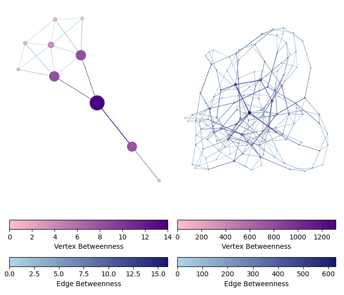
A graph visualizing the betweenness of each vertex and edge. — Krackhardt Kite 图（左）和 150 节点 Watts-Strogatz 图（右）中的顶点和边的介数。边的介数以蓝色阴影显示，顶点的介数以紫色阴影显示。¶

介数的输出如下

vertices: 0.0 - 14.0
edges: 1.5 - 16.0
vertices: 0.0 - 1314.629277155593
edges: 1.0 - 628.2537443550603

python-igraph 手册

Betweenness （介数） ¶

介数¶